TL;DR: the Exclusive Top Floor algorithm is a blazingly fast algorithm to sample arbitrary continuous probability distributions solely from their probability density function (PDF) and using only marginally more than one random number per sample.
A free reference implementation is provided as a C++ library.
Why should I use it?
The ETF algorithm has a number of advantages over other methods, including:
speed: it is comparable in speed to the ziggurat algorithm [1] and thus typically many times faster than inversion sampling,
quality: the entropy of the generated distribution is noticeably higher than that of the ziggurat and quite close to that of inversion sampling; in fact, ETF will even outperform inversion sampling in terms of quality in the common cases where the RNG produces more bits than the precision of the floating-point type used (e.g. 32-bit random numbers paired with single-precision floats or 64-bit random numbers paired with double-precision floats).
convenience: there is no need to know the cumulative distribution function (CDF) and even less its inverse; the lookup tables can be automatically generated with a multivariate newton method provided within the library, requiring only the PDF and its derivative (though even the PDF derivative could be omitted with the use of e.g. a multivariate secant method),
versatility: unlike the ziggurat, it can be applied to a wide range of distributions including non-monotonic or asymmetric distributions; also, the x position beyond which the tail is sampled with a fallback algorithm can be arbitrarily adjusted without consideration for the statistical weight of the tail,
statistically independent samples: unlike Markow chain Monte Carlo methods such as the Metropolis-Hastings and slice sampling algorithms, the ETF method does not introduce correlations between samples.
thread-safety: unlike some distribution-specific methods such as the Box-Muller transform or the polar method, the ETF algorithm is inherently stateless and numerical distributions can thus be safely and efficiently shared between threads (though thread-local RNGs are still required, of course).
So what is the catch?
Although it is unlikely to matter in practice, there is a small space vs speed trade-off: the reference implementation needs 3 floating-point tables and 1 unsigned integer table with typically 128 or 256 elements each.
Also, if the parameters of a distributions are not statically known and the distribution cannot be generated by cheap transformation of a fixed-parameters distribution, then the tables must be generated dynamically. This one-time cost is usually easily amortized, however, since table generation has only Ο(n) complexity and, in the case of Newton’s method, a quadratic convergence rate with respect to precision.
The bottom line: unless only relatively few samples are to be generated, the ETF method is likely to provide substantial benefits with very few downsides.
How does it work?
The big picture
The underlying idea of ETF is simple: a majorizing function for the PDF is defined using adjacent vertically laid rectangles forming a “city skyline”, as in an upper Riemann sums. Instead of splitting the x interval evenly, however, the partition is specifically chosen so that all rectangles have equal areas. A minorizing function is in turn defined with somewhat smaller rectangles laid out on the same sub-intervals. The top floors giving their name to the method are the small rectangular areas filling the space between minorizing and majorizing rectangles.
Using the real estate analogy, inhabitants are initially distributed evenly within the buildings by choosing a location at random within the area under the majorizing function, i.e. anywhere between the ground and the skyline. To do so, a building is first chosen at random (equiprobably since upper rectangles have the same area) and then a random location within that building. If an inhabitant end up on a lower floor, its location is accepted right away without further computations.
If an inhabitant ends up on a top floor, however, he will need to prove that he really belong there: the PDF is evaluated at the vertical of the location to check whether it indeed lies under the PDF, failing which the inhabitant will be expropriated. Staying true to the analogy, the lower floors are therefore (computationally) much cheaper than the topmost floors but fortunately are chosen much more often, thus keeping the average cost at a low level.
Implemented naively, however, this method would still require two or even three random numbers per sample: one to choose the building and two to choose the vertical and horizontal coordinates within the building. The method wouldn’t be very new either [2].
The gory details
So here is how it really works. Let us consider for the sake of simplicity a non-symmetric distribution with compact support. The algorithm starts by computing the majorizing and minorizing functions as outlined above, typically using a partition with 128 or 256 sub-intervals. Ignoring some additional optimizations made in the actual implementation, random variates are generated as follows:
a W-bit random integer is generated,
since all upper rectangles have equal area, a rectangle can be chosen at random from a number extracted from N of the available W random bits (say N=7 provided that there are 128 majorizing rectangles).
the remaining W-N independent bits are used to generate a real number y between 0 and H where H is the height of the upper rectangle,
if y is larger than the height h of the lower rectangle then jump to 6 (wedge sampling, a.k.a. top floor test), otherwise proceed to 5 (acceptance),
[here is the trick]: we are left with y, a nice number uniformly distributed in [0, h) with almost the same entropy as the untested y —we have only lost log₂(H/h) bits— so why throw it to the garbage? Instead, we apply an affine transformation to y from interval [0, h) to interval [xᵢ and xᵢ₊₁) and return the number x thus produced.
[wedge sampling: this happens rarely] another random number x within the current rectangle interval [xᵢ and xᵢ₊₁ ) is generated and y is compared at location x with the PDF envelope; if it is under the PDF, return x, otherwise jump back to 1.
A legitimate question at this point would be whether we have not irremediably lost the N bits of precision used to generate the quantile index.
The answer is no: the generation of x does in fact require less precision since, once the quantile has been determined, the range of possible x values has already narrowed down the interval to [xᵢ and xᵢ₊₁), and since there are 2ᴺ such intervals, one needs this much less precision. In fact, if the function to sample was the skyline majorizing function (i.e. if the top floor rejection step could be omitted), the method could be shown to be nothing else that a (very) fast inversion sampling method without any loss of quality. The overall quality loss is thus in theory relatively moderate and mostly imputable to wedge rejection.
For tailed distributions, the algorithm admits an externally supplied (fallback) tail distribution, just like the ziggurat algorithm; unlike the ziggurat, however, it does not require the area of the tail to be equal to that of the quantiles, thus relaxing the constrain on the x threshold beyond which the fallback tail needs to be used. One may also use instead a majorizing PDF for the fallback and apply rejection sampling in the tail.
To include a tail, step 4 above is modified to generate a real number y between 0 and H/(1-P(tail)) where P(tail) is the tail sampling probability (i.e. the area of the tail divided by the total area of the majorizing function, tail included). If y is greater than H, then the tail is sampled.
Note that for the sake of efficiency, in the actual implementation y is an integer and the various rejection thresholds are appropriately scaled so as to only use integer arithmetic until x is to be computed.
Quality
Quality, qualitatively
The ETF algorithm is RNG-agnostic so potential quality issued related to the RNG itself will not be investigated. Also, since this is a rejection method, goodness of fit is assumed without demonstration.
The main question becomes therefore: how much of the quality of the original RNG does it actually retain? Or alternatively, how “uniformly” (in a loose meaning) would the numbers be distributed if we used an ideal RNG? From this perspective, inversion sampling can be considered the reference method: baring rounding issues and provided that the floating point mantissa has more digits that the random number, one can always map a number generated by inversion sampling back to the original random number using the CDF.
One way to crudely assess the quality is by sampling the distribution with a high quality RNG, using many more samples than the range 2ᵂ of the RNG. If we set for now our ambitions and W low, at say 16 bits, this is fairly easy to do.
Without further ado, this is the result of the collection of 10⁹ normal variates in 1001 bins, generated with the ziggurat and the ETF algorithms with a 16-bit RNG (actually, a truncated MT19937).
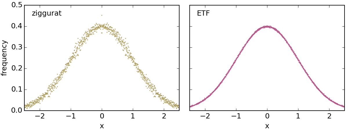
Yes, quite a difference.
It is important to note that these are the converged numerical PDFs: all observable deviations from the theoretical PDF are inherent to the algorithm used and are not related to the RNG: adding more samples or using another (good) RNG would not change these plots in any visible manner. In fact, a testimony to convergence can be directly found in the symmetry of the scatter plots.
Quality, quantitatively
But can quality be assessed in a more rigorous manner, especially at higher precision W? To some extent, yes. A test that can point to poor distribution of the variates at small scales without requiring too much computing power is the Knuth collision test [3] where n balls are randomly thrown into 2ᵈ urns. Even with n<2ᵈ, the number of collisions (i.e. balls that get into an already filled urn) can be sufficient to form the basis for a statistical test that assesses uniformity defects.
Following Doornik [4] we first generate normal variates and then use the normal CDF to transform them back to a random number that should be uniformly distributed in [0, 1). The Knuth collision test is then performed for several values of d, keeping n smaller than 2ᵈ by a factor of 256. The RNG is a MT19937 with W=32 bits and all floating point computations are performed in double precision. The ziggurat and ETF algorithm both use 128-entry tables. The inversion sampling test used for comparison is actually an ideal case: it is simulated by simply transforming the RNG integer directly to a uniform number in [0, 1), which is akin to performing inversion sampling and then transforming back the variate with the normal CDF using infinite floating point precision.
So here are the results, with each test repeated 10 times for each value of d. See the source for details (note that the Boost special functions library is required).
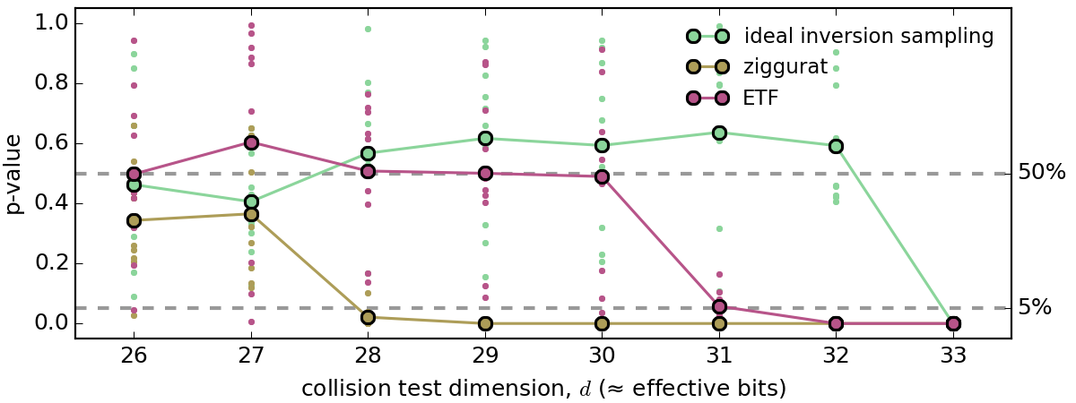
Without going into details, if the variates are well distributed then the 10 p-values (scatter plot) should be uniformly distributed between 0 and 1 and their mean value (solid line) should be close to 0.5. When all p-values go low (the traditional threshold is 5%), this is a sure sign that the test has failed.
So what does this plot say?
Expectedly all algorithms fail at d=33 since with W=32 bits of information it is obviously impossible to evenly distribute balls into 2³³ urns. Simulated inversion sampling succeeds at d=32, but this was also expected since this ideal inversion sampling test is de-facto a measure of the quality of mt19937 (which is known to be good).
The quality of the ETF algorithm is very satisfactory with a loss of only 2 effective bits compared to ideal inversion sampling. The ziggurat algorithm is clearly worse with a 5-bit effective loss compared to ideal inversion sampling, thus confirming the hint given by our former visual comparison of distributions generated with W=16.
Speed
The ziggurat was of course used as the reference algorithm for speed since it is widely considered the fastest method to generate normal variates of reasonable quality.
In order to provide a fair comparison, the ziggurat algorithm used as baseline was also made portable and generic over the RNG precision (parameter W). At the same time, an apparently yet unreported bug in the original ziggurat algorithm which seems to have propagated to many implementations was fixed (see comments in the source code). The original ziggurat algorithm is also benchmarked as a sanity check to make sure that the speed of the corrected and precision-generic algorithm remains comparable.
The ETF implementation reflects most of the feature of the corrected ziggurat implementation but is additionally generic over the number of bits N of the table index whereas the ziggurat was hardcoded with N=7. In order to compare apples to apples, all tests are performed with N=7 for both the ziggurat and the ETF algorithms.
The speed benchmark was run on a i5-3230M (yes I know — I accept donations). It sums 10000 normal variates with either the 32-bit MT19937 (for W=32) or with the 64-bit MT19937 (for W=64) of the C++ standard library as RNG. Each of the reported timing is an average over 1000 tests. Feel free to contribute your timings using the benchmarking code.
| W=32 bits | gcc 4.9.2 (-O2) | clang 3.5.0 (-O2) |
|---|---|---|
| Generic, portable, fixed ziggurat | 71.9 µs | 97.6 µs |
| Original ziggurat | 66.6 µs (-7%) | 95.4 µs (-2%) |
| Exclusive top floor (generic, portable) | 72.7 µs (+1%) | 115.9 µs (+19%) |
| W=64 bits | gcc 4.9.2 (-O2) | clang 3.5.0 (-O2) |
|---|---|---|
| Generic, portable, fixed ziggurat | 80.4 µs | 97.5 µs |
| Original ziggurat | 70.5 µs (-12%) | 95.7 µs (-2%) |
| Exclusive top floor (generic, portable) | 81.4 µs (+1%) | 112.1 µs (+15%) |
| libstdc++ (polar transform) | 437.7 µs (+444%) | 1440.7 µs (+1378%) |
Despite a few oddities like clang taking longer to compute with a 32-bit RNG than with a 64 bit RNG and being in general worse at optimising the ETF, the picture is very consistent: the difference between the baseline ziggurat and the ETF is barely noticeable with a penalty limited to 1% on gcc and 19% on clang, compared to an abysmal +444% and +1378% for the native libstdc++ implementation of the normal distribution which uses the polar transform. Tests with -O3 give nearly identical figures for gcc and actually slightly worse figures on clang for both ziggurat versions as well as for the ETF (by a couple of %), the only gain being observed on the libstdc++ polar transform which drops to “only” 931 µs.
Conclusion
The ETF method generates samples which quality is substantially higher than that achievable with the fastest algorithm to date—the ziggurat method—for a roughly equivalent computational cost and a much greater versatility regarding its applicability to arbitrary continuous univariate distributions.
Todo
Hopefully a Rust implementation will follow. Maybe. One day.
Contributors for ports to other languages are very welcome.
References
[1] G. Marsaglia and W. W. Tsang, “The ziggurat method for generating random variables”, Journal of Statistical Software 5, 1-7 (2000).
[2] R. Zhang and L. M. Leemis, “Rectangles algorithm for generating normal variates”, Naval Research Logistics 59(1), 52-57 (2012).
[3] D. E. Knuth, “The art of computer programming”, Vol. 2, 3rd ed., Addison-Wesley (1997).
[4] J. A. Doornik, “An improved ziggurat method to generate normal random samples”, Technical note, University of Oxford (2005).